KML-KMZ Bugs: For Google Every File is a URL

Recently a friend was struggling with KML-KMZ so called "ground overlays" -- draping local maps and imagery over specific map regions in desktop & mobile application Google Earth.

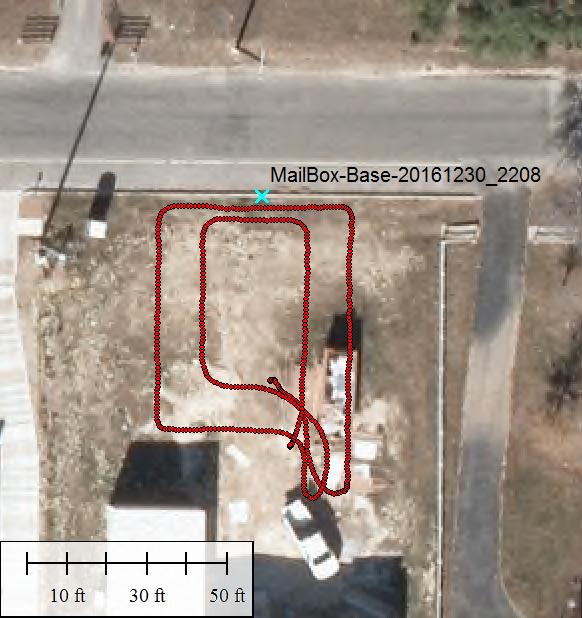
Specifically, aerial data processing via DroneDeploy -- and other photogrammetry apps -- and exported via KML-KMZ data "containers" -- when viewed in Google Earth desktop -- was producing the dreaded BIG RED X -- like this:

Google Earth: Big Red "X" for broken URL links.

Why does this happen? Before we dive into specifics, perhaps it is wise to recognized this key software design premise "baked" into every Google application and product: There are NO "files" on the web -- every file is really a web link.

KML-KMZ RAPID DIAGNOSIS?  Generally two possibilities before we can mental "see" the necessary fix:

(1) Missing local file: The image map overlay is missing from the local computer / mobile device -- or is NOT in the same folder path from which the KML-KMZ was launched (or opened), or,

(2) Busted URL (Universal Resource Locator): The KML-KMZ file contains a "broken link" -- a link that FAILS to point to actual internet "cloud" location.  This broken link can be "busted" by just a single character -- and Google Earth will be clueless -- and paste the Big Red X in the image map overlay space -- signally that Google Earth "knows" some image map *should* be there -- but fetch of the URL failed (404 file not found).

NERD DETAILS:  Opening the "broken" KML file in a plain ASCII or UTF-8 text editor -- GVIM (or MS Notepad ) -- and examining the guts -- we note the key <href> line:

Screenshot: Plain text editor GVIM internal view of 

"busted" KML file and generating Big Red X
(click for bigger)

The "fix" is simple -- from inside a plain text editor -- force the HREF line to "point" to an appropriate image map overlay -- stored -- somewhere -- in the internet cloud.  

Somewhere? Where to store the Google Earth image map "ground overlay"?  Two places -- one the KML-KMZ user can control -- and another that is more "ownership" problematic over the long term (months to years):

(1) Private Web Server w/ Public Exposure: Store the image map overlay on your personal web server -- a web server that exposes a PUBLIC link the world wide web.  For this author: Upside? This is a preferred method -- as "ownership" and control is well defined.  Downside? Requires build or purchase of a web server (i.e. Blue Host, Hostgator, Linode or Tektonic or related).

(2) "Public" web server: Store the image map overlay "in the cloud" -- and with publicaly exposed "hard" link that "reaches" into Google Photos -- or Imgur -- or Amazon S3 -- or some other "photo sharing" website -- THAT CAN AND WILL EXPOSE a "permanent" public link with *NO* demands for "log in." (The big offender here is Facebook and others attempting to enforce viral marketing of their "walled garden").  

CRAZY and OBSCURE LINKS: "Cloud Storage" w/ commercial vendors like Google -- or Imgur -- or Amazon S3 -- is tricky -- because "permanent" and hard links are kinda wild and tricky to determine and extract for use in human edited-updated KML-KMZ files.  Example -- for this topo image map we examine how stored in Google Blogger:

1976 USGS Topo Map "image overlay" for 

Cibolo Nature Center near Boerne TX
(click for full resolution)

The public, "permanent" link looks like this wild mess :

https://blogger.googleusercontent.com/img/b/R29vZ2xl/AVvXsEi0cNC7K7VEpK-PRj8Z_vmULcTGb8X5TNMMt-502WhLDmjvyFP2Ww041Bm0cjnrSIkj2v5VenCSMMZLkxOplckG6nflSX9nmTBsFtJlGyDKBy6xX0HK500K-I03u73DldGL788CsakpE2A/s1600/cibolo_nature_usgs_topo_1976_83dd_v0.png

(makes sense to a web browser or mobile app -- bizzare to any human eye not attached to nerd programmers)

Why so ugly? Google Blogger is "storing" the image map overlay in some deep database index that only makes "sense" to your browser or web app -- and the "Google System."
  
MIXING THE MAGIC: How to FIX the BIG RED X?  And use Google "cloud storage" inside this KML?  Edit-update the KML-KMZ file -- so that the HREF line utilizes the big ugly Blogger image link of above (or a "simple" URL on your personal web server).  Specifically for this example:

Corrected KML file with wild, long and 

ugly "permanent" URL link into Google

Blogger "cloud" storage (click for bigger)

SUCCESS?  First a Google Earth screen shot:

1976 USGS Topo image map ground overlay

properly draped inside Google Earth and 

over Cibolo Nature Center near Boerne TX
(click for bigger)

And click (or tap) this link to view the "live" KML file inside Google Earth.

SUMMARY:  In order to MAX SHARE DroneDeploy and other "cloud processed" aerial imagery data products -- exported via KML-KMZ "containers" -- the key image map overlays must be stored "in the cloud" -- with "permanent" and hard public links.  Google KML-KMZ inherit the Google design premise that every file is really a web link or URL.

Good luck!  And happy value hunting via data explorations!

Solar Eclipse 21-Aug-2017 & Lizard Brain Surprise

Solar Eclipse 21-Aug-2017?  Only 61% Occultation?

Ho-Humm: I was slow to become excited about today's solar eclipse across the USA. After all -- what was the great mystery in a shadow crossing the earth?

But sometimes it is the little things that wake up a child like wonder and thrills.  And trigger surprise emotions & non-verbal brain signals from my Lizard Brain

Hours before the predicted solar eclipse max -- I did spend 25 mins building a shoebox "telescope" -- a miniature Camera Obscura for indirect observation of the 61% max solar eclipse shadowing south Texas.  

Camera Obscura Woodcut from Wikipedia

And I was enjoying eclipse 2017 geographical progress via video coverage on NASA TV Live via YouTube.  

One Possible NASA TV Live Logo

SURPRISE and AWE: But my interest and child like wonder -- and my Lizard Brain "triggers" -- these really peaked when I first stepped outside to test my shoe box "telescope" -- and looking down -- realized there was something really different: Countless magical Solar Crescents: Every sunbeam thru the trees was transformed into a little wonder of nature! Perhaps a photo to illustrate.

Stepping out to test shoebox "telescope and seeing

every sunbeam transformed into a Solar Crescent

INTELLECT vs LIZARD BRAIN: Yes, a solar eclipse seems trivial from an intellectual viewpoint. But your lizard brain is kinda surprised & startled when you realized something is very different about every sunbeam thru the trees.  This surprise emotion suggest why solar eclipses are so emotional for some -- and were great sources of terror in the past: Every part of our being is "hard-wired" to expect & assume the Sun is daily round -- and reliable.  When the Sun is not round & reliable -- the Lizard brain starts talking in brain signals -- under the surface of our conscious minds -- where words rarely traverse.  

Lizard Brain?  Perhaps an vehicle driving example.  On long road trips with little traffic -- your mind gets bored. Soon you are observing the passing scenery or listening to an interest radio program. 45 mins later -- you "wake up" and realize you have been driving -- with success -- no wrecks -- yet you cannot recall any specific driving details of the last 40-60 miles.  No specific conscious decisions about curves or speed or lane changes.  In essence -- the Lizard Brain "took over" the driving from your conscious mind -- a biological "autopilot."   Your conscious mind is only "called up" by the Lizard Brain -- if some driving problem manifest that was "too difficult" for the routine auto-pilot decision loops of the Lizard Brain.

MORE VAGUE LEARNING: Your Lizard Brain can and does learn many thinks -- often without specific, conscious instruction. Example? Do you recall learning how to crawl or walk or drink?  You did learn -- but now these skills are "just in there" -- "hard wired" -- deep into your Lizard Brain and body.

Solar Eclipse and Your Lizard Brain?  And your Lizard Brain is learning thousands of other daily details that almost never "boil up" to your conscious mind.  Many are "environmental triggers" for what is "normal" and "odd" -- environmental details that often keep us out of trouble & alive.  This included an unconscious "awareness" of how the Sun & Moon and stars "should be" on a regular basis.  And an unconscious awareness of what are "normal" sun shadows -- and when this normal is "broken" -- by what might be a danger or predator above us in the sky.

UPSHOT:  I was surprised by my internal emotional reaction to the crescent sunbeams thru the trees.  My Lizard Brain communicated -- not in words -- but via unspoken emotional triggers -- that something was "spooky different."  These emotional signals were BEYOND words and independent of my intellectual understand of the solar eclipse event.

As I reviewed my Solar Eclipse 2017 videos -- I caught myself "giddy" in my voice dialog.  As I thought back the many total eclipse sites covered on NASA TV and other TV networks -- and mixed reactions of folks on the ground -- their emotional reactions were surprisingly genuine and unforced.  Some just fell silent in the total eclipse darkness:

CBS News from Jackson Hole Wyoming,

On camera talent's genuine loss for words in

almost 100% total darkness.

(3 min 22 sec clip)

Some became giddy or child like in verbal expressions.  Based upon my experience -- I would bet that deep wired Lizards Brain reactions to the Sun going dark affect everyone -- in ways that surprise even the most careful & controlled internal conscious observer.

Below are a few simple videos from today.  Those who know me well can judge for themselves if my Lizard Brain was over stimulated.

Solar Eclipse at 61% & Shoebox 

"Camera Obscura" in Operation

Ad Hoc "Colander Telescope" and a

Solar Crescent from every hole.

Solar Eclipse 2017 at 61% Max Occultation

and countless Solar Crescents in every shadow

Enjoy!

Solar Eclipse 1918 Vestigial Memory vs 2017 Internet

Here is an odd three generation Syzygy -- an astronomical "connection" across three generations.  Cross Generational "memory" -- in an odd way: The Solar Eclipse of 08-June-1918 vs 21-Aug-2017

08-June-1918 Solar Eclipse painting by Howard

Russell Butler (from Wikipedia)

Take notice -- you genealogy searching fiends -- even astronomical events can "index" generational "knowledge" -- of time, place and perspectives.  Transcend living memory -- in and odd ways.

MOON ATE THE SUN in 1918?   As early teen -- back in the 1970s -- on a long road trip -- my maternal grandfather described how scared he was -- as a small child in Arkansas -- when the Sun began to go dark -- and the air grew cold on a full summer June day -- the wind shifted -- a few bright stars came out -- and the chickens began to goto roost -- and the cows drifted to the barn for milking.

My grandfather described how he was playing in the fields -- and ran home in a panic -- only to find his mother -- my great grandmother -- calmly standing on the porch of their simple wood cabin -- with two chunks of paper board -- one with a center pin hole -- and another unmolested -- watching a small bright dot shape shift.

My grandfather asked "What's going on Momma?" -- and she replied that the Moon was "eating" the Sun -- words that my grandfather could understand at the tender age of 8 or 9.  The Moon was casting a shadow across rural Arkansas. This was very rare.  My great-grandmother had read about the upcoming 1918 Solar Eclipse event in the local newspapers -- and constructed a crude "telescope" -- as described in one of the newspapers.

My favorite 1918 solar eclipse find, published in

Denver Post (from GreatAmericanEclipse.Com )

Key map detail? In 1918 my grandfather lived just 

south of "A" in ARKANSAS label - near line of totality.

How so?  How could old paper newspapers "know" that a solar eclipse would unfold?  Short answer:  Solar eclipse events are "hand calculable" -- centuries into the future -- and into the past.  Such is the stability of the Moon's orbit about the Earth -- and when the Moon will block the Sun.  Number crunching nerds have been "predicting" solar & lunar eclipse events since before the ancient Sumerians and Aztecs.

REAL or TALL TALE Memory?  For years -- my grandfather's verbal description of his childhood solar eclipse bugged me -- especially since my grandfather was such a big story teller -- and tended to blow things out of proportion -- just for humor & mischief.

THE INTERNET and SEARCH ENGINES -- One day it dawned on me -- "Hey, I can search for any full -- or partial -- solar eclipse across Arkansas in early 20th Century!" -- in a few mins of searching -- the following links -- with glorious "back calculated" pixs and maps -- came up.  How do I know this is "the eclipse"??  My maternal grandfather was born -- as he said "In 1909 -- way out back in the woods!" -- so a 1918 eclipse would make my grandfather a child of 8 or 9 -- mentally old enough to record a solar event.

80 Sec Video, very good Photo-Realistic simulation of

21-Aug-2017 solar eclipse. Note how stars come out.

STRANGE?  There is something odd -- for me -- looking at these 1918 solar eclipse maps:  I can pin-point -- both in time and map space -- where my grandfather was in June 1918 -- almost to the minute.  Kinda like having a Mr Peabody "way-back" machine -- where we can set the dials -- and go see the past.

Fun additional fact?  The 1918 Solar eclipsed was used to test for gravitational deviation of star light -- by the Sun -- as proposed in Albert Einstien and his theory of general relative.

NOW in 2017: In the lower 48 states -- we have opportunity to experience a very similar eclipse -- on 21-Aug-2017.  A chance to anchor some memories -- and share an immutable event with those that follow.   A few links follow -- with kewl graphics and charts -- to "tickle" your fancy.

Very kewl predictive map for 21-Aug-2017

Solar Eclipse (click for larger, from website

StaryNightEducation.Com )

UPSHOT?  Even poor white trash from Arkansas can "anchor" history -- with not-so-tall tales -- and a little ex-post-facto astronomical research.

Useful links and videos:

[1] NASA Count Down Timer to Live Eclipse 21-Aug-2017

[2] Wiki maps & pixs for 21-Aug-2017 Solar Eclipse

NODATA Data Ghosts in the Machine? $23 Quadrillion Explosions?

The 2004 Movie "I-Robot" starring Will Smith rechewed a 1940-1950s Isaac Asimov story line.  But with a new idea injected the character Dr Alfred Lanning: Ghosts in the Machine -- random snips of code (ad hoc algorithms) that manifest new, sometimes good -- sometimes bad -- behaviors.

I-Robot First edition cover, by Isaac Asimov, 

circa 1940-1950 from Wikipedia

Q: Do ghosts reside in our circa 2017 machines?  Always caused by "random snips of code"?

A: YES -- with a surprise twist:  The "ghosts" are buried in how NODATA tokens are stored -- and interpreted. The ghosts are not in the software -- but in the DATA -- specifically how human software developers adopt unconscious & unknown software ASSUMPTIONS regarding current & historical use of NODATA tokens.

VIDEO: Perhaps a scary $23 quadrillion dollar billing example -- to kick off this significance of NODATA assumptions -- and software interpretations. In 2009, Josh Muszynski of New Hampshire was "billed" over $23 quadrillion dollars via his debit card:

2 min video: Josh Muszynski of NH reviews his online bank statement 

and astronomical $23 quadrillion bill (from WMUR-TV, video alternate link )

Wow!  And the open literature suggests there were some 12,000 other similar example that have gone unreported [1].

Q: How did a NODATA "ghost" cause this surprise bill?  A bill that was over 2000 times larger than the US National Debit in 2009? (or said another way, Mr Muszynski -- if he had actually received the $23 quadrillion -- could have "paid" the US debit and had 1999 extra US-sized debts to spare).

A: The best explanation comes from how ASCII "blank" data (space-bar characters) are "padded" into the debit / credit card reader -- at your local corner store -- and then "digested" by the computers at the bank end.  From a very short illustration [2] from programmer website TheStackExchange:

Q: "Is 23,148,855,308,184,500 a magic number -- or sheer chance?"
A: "Add the cents to the number and you get [19 digit number]: 2314885530818450000 -- which in Hexadecimal [base-16] is: 2020 2020 2020 1250.  Do you see the pattern? The first six bytes have been overwritten by spaces (hex 20, dec 32). "

KEY IDEA?  MESSAGE?  How NODATA is stored -- and interpreted by software and programmer algorithms -- is REALLY, REALLY important.  Failure to recognize interpretive difference between NODATA storage types will make the ghosts pop out of the machine!

References:
[1] Apparently there are some 12,000 other un-reported $23 quadrillion dollar billing errors from NODATA padding & improper interpretation:
http://www.nytimes.com/2009/07/23/nyregion/23towns.html

[2] StackExchange Q&A: Is $23,148,855,308,184,500 a "magic" number?
http://stackoverflow.com/questions/1133581/is-23-148-855-308-184-500-a-magic-number-or-sheer-chance/1139230

Centimeter Grade Differential GPS/GNSS for under $750 !!

Wow! Amazing how technology changes!  GPS Theory & Field Practice are same, but hardware & software light years better!  A quick look from rapid training & GPS-GNSS post processing workflow capture.

Centimeter grade "Reach GPS" Postage Stamp size unit with uBlox
GNSS chipset side up (Intel Edison "WiFi webserver" chip on reverse)

Quick Facts & Links for the time compressed:

• HARDWARE: Centimeter resolution differential GPS-GNSS with two powerful "Reach GPS" postage-stamp boards for under $700 !!  See Reach GPS Intro Page and Reach RTK Starter Kit for under $700 US


• SOFTWARE: Post Process on a $300 WiFi laptop using open source RTKPOST / RTKLIB by Mr Tomoji Takasu.  See GITHUB Page README file or see Source Archives

HISTORY & SIGNIFICANCE: For those of us who first saw "survey grade" GPS back in 1994 or so -- hardware cost was massive money -- $50K to $250K -- and software was steep learning curve. And there was NO GOOGLE to search for online help. Months to years to come up to speed & generate centimeter repeatable results. Reading fat and strange strange technical manuals [a real life 1995 example]. And you needed to be a jack-of-many trades just to get started -- math hero, software guru, electronics nerd, signal processing engineer, entry level orbital mechanics master, etc.  The list of cross-skills seemed endless.  

The author in 2000 with Novatel GPS-Station as

rover & 5.0 meter stadia pole to clear trees and 

gain solid L1 and L2  carrier phase tracking

By 2003, "survey grade" GPS was $25-50K -- and a little more "push button" plug and play.

Circa 2002-2003, Leica 500 on Tripod

Now in 2016?  Wow!

RECENT HISTORY: During 2016 Christmas to year's end "dead time" -- I was helping some UAV friends document & transfer a GNSS post processing workflow -- and was forced -- in a fun way -- to learn both "Reach GPS" and RTKPOST-RTKPLOT (based on RTKLIB).

LOCAL BASE EXAMPLE: Map picture is worth 1000s of nerd words.  First a quick test "flight" where guru Ian Gates hiked the UAV rover around the edges of the driveway, concrete edges and paving lines for visual & repeatable ground tracks.  The "MailBox" was the local reference station -- and was "fitted" with a "ReachGPS" unit -- acting as "Base" and recording local fixed observables. Pictured here are process Lat-Long path from plain ASCII text POS file -- generated as output by RTKPOST:

2013 six-inch aerial photo: Red "flight"/ground track 

of UAV "Reach GPS" Rover along edges of driveway 

& concrete. Note that driveway was under construction 

in 2013 (see KML file here for Google Earth compare 

[careful GE "aerials" are not always "good"])

DISTANT BASE EXAMPLE:  The above UAV Rover set was post processed -- a second time -- via RTKPOST -- and this time using a "distant" (about 5Km) CORS Permanent GPS reference station TXBO (OBS files here).  Resulting map was a bit different -- for reasons that shall become clear:

Same 2013 six-inch aerial: Green is Reach GPS "flight"/ground 

track of Rover along same edges of driveway & concrete. The 

green track is offset approx 4.65 feet SW-NE from red track. 

Again please note that driveway was under construction in 2013. 

(for green track compare in Google Earth, please see KML file)

WHY DIFFERENT?  What caused the approx 4.65 foot offset SW-NE?  After running a dozen RTKPOST sessions -- testing "personality" CONF parameter effects on RTKPOST -- this accident of fast training became apparent -- a difference in the "best guess" for MailBox reference station -- extracted from debug of *.POS outfiles from RTKPOST:

RED Ref XYZ: 29.793639547 -98.719151454 407.6388 (degs/degs/meters)
GRN Ref XYZ: 29.793631843 -98.719162737 404.8325 (degs/degs/meters)
Delta Diffs:  0.000007704   0.000011283   2.8063 (degs/degs/meters)
Cart Offset:  1.52(m) or 4.98 feet
Great Circle: 1.38(m) or 4.53 feet

Note the delta differences: These very closely match GIS/Map plotting SW-NE offset measurements from POS file overlay on aerials.

File Sources: The above XYZ (Lat-Long-Hgt) coordinates were extracted from RTKPOST files:

1. "Rov_201612302215_MailBox_vs_Flite_v2.POS" (red) and
2. "Rov_201612302215_MailBox_vs_Flite.POS" (grn).

UPSHOT? Results?

• This is BIG: RTKPOST combined with "ReachGPS" can "see" consistent UAV flight and/or ground track differences of 4-5 feet.  This is amazing for L1 code only GPS-GNSS receivers.  Take away? With a little less time compression, it is clear from RTKPOST behavior that much tighter solutions can be obtained.
• Trash is Treasure -- Training "Errors" from ref station XYZ entry produced UAV rover repeatable results across different computers and using slight variations in the CONF personality run file (elev angle cutoff, mix of GNSS source signals, sky position blockage, multipath, etc).  Take away? With a little care, RTKPOST is robust.
• Red vs Grn?  Bad vs Good? No, not at all.  Just a way to keep track of which was the "original" run by guru Ian Gates -- and which was run by this author in "trainee" mode.
• Compared to "high end" post processing workflows like GIPSY-OASIS / GAMET / GLOBK RTKPOST is "easy to use" and more or less "intuitive" (if you can see the GPS signal processing theory in your "mind's eye").

Stay tuned for more soon.  Enjoy, RM

Bexar County Texas and Parcel Size vs Counts

Parcel Sizes vs Parcel Counts

Recently a question arose -- in the search for suitable real estate properties vs parcel size -- coupled with ample choice.  
The question was simple:  How many land parcels of a certain size are available for real estate development -- and re-development?

Bexar county TX provides an interesting study and test environment -- over 600,000 well defined tax parcels from the Bexar County Tax Appraisal (BCAD) GIS system.

In this post, I shall examine how parcel sub-division across an urban area trends in a pattern typically seen in language & word complexity -- and mimics something called Zipf's_Law -- and maybe something called Rank_Size_Distribution for city population vs country size ranking.

Rank-Order Distribution for Cities 

(from Wikipedia)

First, the Numbers

The decreasing number of large tax parcels is very noticeable via this "raw" data table extract from the BCAD GIS parcel quilt:

===========================
======= Table 1.0 =========
-------------------  ------
Acre-Range            Kount
-------------------  ------
10000.00 and Up           1
 5000.00 - 10000.00       2
 2000.00 -  5000.00       6
 1000.00 -  2000.00      17
  500.00 -  1000.00      36
  200.00 -   500.00     228
  100.00 -   200.00     545
   50.00 -   100.00    1131
   20.00 -    50.00    3142
   10.00 -    20.00    5284
    5.00 -    10.00    7760
    2.00 -     5.00   16591
    1.00 -     2.00   21665
    0.50 -     1.00   33188
    0.20 -     0.50  172027
    0.10 -     0.20  305560
    0.05 -     0.10   24289
    0.01 -     0.05    6995
     Less than 0.01    3094

The above table matches what life experience tells us:  Small parcels are common with large repeat counts; Large parcels are rare.  And because Bexar county is mostly an urban area -- there are a large number of "individual" sized lots -- mostly for residential and small biz operations.

The lone parcel above 10,000 acres in 2015 BCAD tax parcel  quilt was 31062 acres for Camp Bullis military reservation.  Many of the largest parcels are "tied up" by utility, quarry, water & sewer treatment operations, public green spaces, quasi-government entities and military bases & industrial parks.

For Bexar county, the most common tax parcel (lot) size was between 0.10 and 0.20 acres -- 4456 to 8712 square feet -- corresponding to square lots of about 66x66 feet to 93x93 feet.  An examination of the GIS parcel quilt confirms this large count corresponds almost exclusively to single home lots and residential areas.

Trend Surprise?

A log-log plot of Table 1 (above) produced some interesting kinks and hints:

Fig 1: Bexar Acres vs Count

(click for larger)

Dots in Fig 1 plot are the observed acres vs counts from the 2015 BCAD GIS.  

MATH MODEL? Assuming the observed data might "follow" a "power law" relation of the form:

y = a x ^b

The blue and red lines are two possible mathematical "fits" to the observed data.  WHY?  For what purpose?  To extract some numerical "intelligence" and "insight" from the data.  Sometimes "math models" provide hints of related data patterns from seemingly unrelated subject areas.

BLUE LINE was a least squares "fit" to the data from 0.5 to 31062 acres -- and manifests a "fit" to the following "power law" relation:

parcel_count = 45305 acres ^-0.9774

The coefficient 45305 is interesting because it is "close" to the Camp Bullis large acreage -- which dominates the rank-order distribution of tax parcels.  The exponent "-0.997" is close to "-1.0" -- which means that tax parcel acreage vs counts is an inverse relation -- i.e. like this equation:

y ~= 1/x

RED LINE also assumes a power law relation -- and uses the Camp Bullis acreage of 31062 acres as the "y-intercept" and "origin" for the decreasing counts -- as acres increase. Also, assuming that observed data has a strict inverse relationship:

count = 31062 acres ^-1.0

or using algebra:

count = 31062 ÷  acres

SIGNIFICANCE?  The odds of finding a large parcel in Bexar county goes down -- rapidly -- in a pattern that mimics Zipf's law for complexity of words in language.  This is also similar to the odds of large cities in countries of various sizes.

Where Does Land Value Live?

VALUE DIG HISTORY -- Back in 2005, I had a real estate investment client who asked this rough question:

  "Hey, where does *REAL* land value 'LIVE' in Kendall County Texas?"

With the added conditional:

  "And don't give me those appraisal 'compares' -- they are just made up by some guy at tax office."

The actual question was bit more complex -- yet basically boiled down to the above question and conditional. 

KEY PURSUIT -- This "real" value question drills down almost to the core mission of this blog: "How do we know -- what we think we know!"  This posting will tickle the edges for key insights.

Mission Probable: 

Buying the Desired Answer?

SALES vs TAX APPRAISAL -- It is true that most property tax appraisal districts "make up" some -- but not all -- of the property values.  Recent and past "actual" sales are also used to help determine changes of property "value."  The key difference?  And this was buried in my client's question -- how to DISTINGUISH "real" sales values from "made up" values for tax appraisal purposes.  Was there a method to pull these different kinds of value apart for examination?

'MARK TO MARKET' PROBLEM -- Sales Trends vs Long Term Holdings and "Pollution" of values. 

To be more fair to tax appraisal districts -- consider the long term value trend identification issue: For some properties -- that remain in the same hands for 10 / 20 / 40 years -- and fail to manifest a "real market price" -- via a realized market sale -- and in order to collect "fair and balanced" tax values -- tax appraisal districts must "guess" the property value for taxes -- roughly every year. 

While the guess (estimation) process is heavily vetted and subject to many rules -- and in most tax jurisdictions attempts to be "fair" and "reasonable" -- the estimation process can be biased -- either accidentally -- thru blunders or poor attention to details -- or for more mischievous reasons (for revenue / political influence).  "Vet" and "Zen" of "real" property value verses price Skullduggery can be tricky to identify -- when just looking at one to 10 lots in the field.  Sometime larger patterns can be "seen" when a few 1000 parcels are compared -- via one possibe approach -- outlined below.

Skullduggery?  Yes, who can "out-guess" the official "guesser" for a property "value?"   Whether the "guesser" is "official" or "consultant" -- the raw tax data routinely fails to identify the guesser's orientation -- and the bias factors will change from year-to-year -- and decade-to-decade.  A "price bias" -- either high or low -- can remain in the data for many years.

LAST SALE OVER-RIDE -- Some county GIS tax databases *do* flag "real" sales vs some other valuation process -- and will sometimes report a "last sale" date -- presumably to trigger some "superior" valuation process -- like "Hey, this tax value is too old -- we need an updated estimate for next year's appraisal."   

However -- not all county tax GIS-databases retain "last sale" information -- and if retained -- there are no guarantees the "last sale" dates are realistic or were maintained in a careful manner.  Plus an adjoiner sale value -- *NOW* -- will often influence or over-ride any past considerations.  Experience with tax appraisal databases from AK / PA / LA / ND / NM / TX / and others -- indicate "last sale" maintenance -- and tax value significance -- varies much from county-to-county -- and state-to-state (much seems to depend on local tax jurisdiction policies, "personality,"  data absorption and appraisal skills).

UPSHOT?  REAL GOAL? -- My client wanted to DIFFERENTIATE between a "real sale price" -- verses -- systemic valuation bias (i.e. county wide guesses) in the reported property values.   My client wanted the "data behind the data" to aid his investment search.

RAW DATA and QUICKLOOK -- GIS data was obtained from a public source for Kendall county Texas (KCAD Data).  The data was "fresh" and up to date -- in the sense that a very dedicated and skilled GIS camper had brought the KCAD tax data -- and the parcel data -- up to good digital standard.  

Review of the data -- and "testing" on an "example" sub-division -- produced an interesting 1st cut surprise.  Maps and details to anchor the eyeballs and brain for "Alamo Springs" 

2004 Kendall County TX Parcel Map

and Location of Alamo Springs in Green

(click for larger)

And a Log-Log Plot of the raw ACRES (x-axis) -- verses -- "Sale or Tax Value" (y-axis) yielded an interesting scatter plot pattern:

Log-Log Value Chart

Acres (x) vs Sale or Tax Value (y)

Green Dots: Alamos Springs Parcels

(click for larger)

Dot Value-vs-Color Legend

1ST BRUSH SIGNIFICANCE -- The clustering of Alamo Springs sub-division parcels (green dots) along the X-axis was no surprise -- in year 2004 -- the sub-division "lots" were roughly between 2 and 15 acres.  

The clustering in dollar value -- along the Y-axis -- was more interesting -- especially when "compared" to other parcel valuations across the county (blue to red dots):  The lot values were scatter clustered between $10k and $100k -- and were "stabbed" by a lower-left to upper-right linear clustering line pattern.  

This linear clustering pattern was found -- via stats and regression analysis -- to generally be along a trend line of approx $7000 per acre.  Rough descriptive trend equation was found to be of the form:

  Value (dollars) = $7000 x Acres^(-0.98)

Where the exponent of Acres -- the value "-0.98" -- is very close to "-1.00" -- and where a negative 1.0 exponent means "per acre."

Other trend lines -- above and below -- were also expressed -- and numerically explored.  These trend line scatter patterns suggested some "hidden hand" in the property market was "setting" land value vs acres in some deliberate and mathematically deterministic way.  My client wanted to know:  Was this trend line from tax appraisal estimated values?  Or a "real" market "signal" in sale prices?  A trend that could be leveraged for better "buy in" decisions.

DOTS with ID -- Each of the Log-Log scatter plot dots were "addressable" -- and each dot had a "link back" to the original parcel data attributes -- parcel ID number, landowner name, last sale date, land acres, improvements, etc.

VALUE SPACE QUERY FOR REAL SPACE LOCATION -- In short -- and this is the key point of this posting -- dots on the Log-Log value chart could be interrogated in Log-Log space -- and the significance of their map geo-location -- if any -- could be determined.  Basically a rapid technique for flipping back and forth between "comparables" -- in terms of land value -- to map location -- and noting any significant acre-vs-value patterns.

1st TEST -- SMALL ACRES, MEDIUM VALUE Compares -- My client wanted to examine small acreages -- usually highly developed and in urbanized "towns" -- verses -- the much more ranch-land rural parts of Kendall county.  Some more surprise -- a Value-vs-Acres selection -- in the Log-Log chart space -- like thus:

Chart: "Value" Selection in Dollars 

vs Acres in Log-Log Scatter Cluster Space

(click for larger)

MANIFEST IN THE "MAP SPACE" -- This blob selection "Lit Up" the Kendall county parcel map -- in yellow -- thus:

Kendall County Map: Parcel Selection by

1st "Blob Query" in Log-Log Value Space

(click for larger)

INTERESTING POINT -- The Log-Log selection blob "found" parcels -- on the map -- that were generally in urban and "developed" areas.  Lots located in the towns of Boerne and Comfort Texas.

2nd TEST - LARGER ACRES, MEDIUM VALUE Compares -- Searching for a "Bargain" property.  A second "Blob" selection in the Log-Log value space "found" Kendall parcels in very different map locations:

Chart: "Value" Selection in Dollars 

vs Acres in Log-Log Scatter Cluster Space

(click for larger)

IN THE "MAP SPACE" -- This 2nd blob selection "Lit Up" the Kendall county parcel map -- in yellow -- for larger sub-division areas -- outside the "town" areas:

Kendall County Map: Parcel Selection by

2nd "Blob Query" in Log-Log Value Space

(click for larger)

MYSTERY COMPARES -- Significant Outliers -- In the Log-Log value space plots:  There were other, more mysterious "offset" points -- out near the edges.  The best example called out in the charts:  the Benedictine Sisters Orphanage located on the former Kronkosky property -- a significant outlier with a very large valuation:  Approx $19.6 million for some 40 acres -- $488,400 per acre in 2004.  This large valuation would make NO fiscal sense for a private landowner -- as the taxes would be out of proportion for offset "comparables."  However -- since the orphanage is a charity -- and probably tax exempt -- there would be no tax bill.

Negotiation Leverage?  One possible interpretation for this significant outlier?  Sharing this example with various appraisal experts -- the speculation?  This large valuation is used to self-report and to establish a trend:  In the event the orphanage is forced to sell -- eminent domain or related for public space, road or utility corridor -- or chooses to sub-divide and sell a lot or two -- the orphanage negotiators can begin with a very high price history -- and appear price flexible -- as the negotiations unfold.

SUMMARY -- The above Log-Log value space analysis has been repeated for Bexar County Texas -- a county with approx 600,000 parcels -- with some surprisingly similar results -- and some unique differences.  Because Bexar county is "more urban" -- and more "mixed use" than Kendall county -- Value space chart patterns are very different for Bexar county -- and exhibit many "localized" value personalities.  Stay tuned for a future example.