Where Does Land Value Live?

VALUE DIG HISTORY -- Back in 2005, I had a real estate investment client who asked this rough question:

  "Hey, where does *REAL* land value 'LIVE' in Kendall County Texas?"

With the added conditional:

  "And don't give me those appraisal 'compares' -- they are just made up by some guy at tax office."

The actual question was bit more complex -- yet basically boiled down to the above question and conditional. 

KEY PURSUIT -- This "real" value question drills down almost to the core mission of this blog: "How do we know -- what we think we know!"  This posting will tickle the edges for key insights.

Mission Probable: 

Buying the Desired Answer?

SALES vs TAX APPRAISAL -- It is true that most property tax appraisal districts "make up" some -- but not all -- of the property values.  Recent and past "actual" sales are also used to help determine changes of property "value."  The key difference?  And this was buried in my client's question -- how to DISTINGUISH "real" sales values from "made up" values for tax appraisal purposes.  Was there a method to pull these different kinds of value apart for examination?

'MARK TO MARKET' PROBLEM -- Sales Trends vs Long Term Holdings and "Pollution" of values. 

To be more fair to tax appraisal districts -- consider the long term value trend identification issue: For some properties -- that remain in the same hands for 10 / 20 / 40 years -- and fail to manifest a "real market price" -- via a realized market sale -- and in order to collect "fair and balanced" tax values -- tax appraisal districts must "guess" the property value for taxes -- roughly every year. 

While the guess (estimation) process is heavily vetted and subject to many rules -- and in most tax jurisdictions attempts to be "fair" and "reasonable" -- the estimation process can be biased -- either accidentally -- thru blunders or poor attention to details -- or for more mischievous reasons (for revenue / political influence).  "Vet" and "Zen" of "real" property value verses price Skullduggery can be tricky to identify -- when just looking at one to 10 lots in the field.  Sometime larger patterns can be "seen" when a few 1000 parcels are compared -- via one possibe approach -- outlined below.

Skullduggery?  Yes, who can "out-guess" the official "guesser" for a property "value?"   Whether the "guesser" is "official" or "consultant" -- the raw tax data routinely fails to identify the guesser's orientation -- and the bias factors will change from year-to-year -- and decade-to-decade.  A "price bias" -- either high or low -- can remain in the data for many years.

LAST SALE OVER-RIDE -- Some county GIS tax databases *do* flag "real" sales vs some other valuation process -- and will sometimes report a "last sale" date -- presumably to trigger some "superior" valuation process -- like "Hey, this tax value is too old -- we need an updated estimate for next year's appraisal."   

However -- not all county tax GIS-databases retain "last sale" information -- and if retained -- there are no guarantees the "last sale" dates are realistic or were maintained in a careful manner.  Plus an adjoiner sale value -- *NOW* -- will often influence or over-ride any past considerations.  Experience with tax appraisal databases from AK / PA / LA / ND / NM / TX / and others -- indicate "last sale" maintenance -- and tax value significance -- varies much from county-to-county -- and state-to-state (much seems to depend on local tax jurisdiction policies, "personality,"  data absorption and appraisal skills).

UPSHOT?  REAL GOAL? -- My client wanted to DIFFERENTIATE between a "real sale price" -- verses -- systemic valuation bias (i.e. county wide guesses) in the reported property values.   My client wanted the "data behind the data" to aid his investment search.

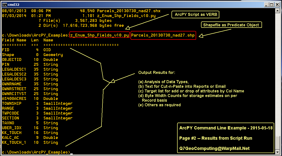
RAW DATA and QUICKLOOK -- GIS data was obtained from a public source for Kendall county Texas (KCAD Data).  The data was "fresh" and up to date -- in the sense that a very dedicated and skilled GIS camper had brought the KCAD tax data -- and the parcel data -- up to good digital standard.  

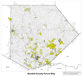
Review of the data -- and "testing" on an "example" sub-division -- produced an interesting 1st cut surprise.  Maps and details to anchor the eyeballs and brain for "Alamo Springs" 

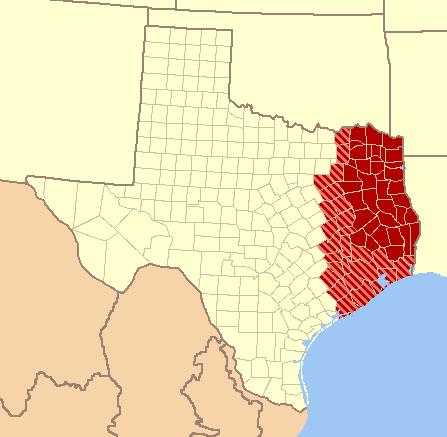
2004 Kendall County TX Parcel Map

and Location of Alamo Springs in Green

(click for larger)

And a Log-Log Plot of the raw ACRES (x-axis) -- verses -- "Sale or Tax Value" (y-axis) yielded an interesting scatter plot pattern:

Log-Log Value Chart

Acres (x) vs Sale or Tax Value (y)

Green Dots: Alamos Springs Parcels

(click for larger)

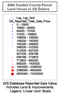
Dot Value-vs-Color Legend

1ST BRUSH SIGNIFICANCE -- The clustering of Alamo Springs sub-division parcels (green dots) along the X-axis was no surprise -- in year 2004 -- the sub-division "lots" were roughly between 2 and 15 acres.  

The clustering in dollar value -- along the Y-axis -- was more interesting -- especially when "compared" to other parcel valuations across the county (blue to red dots):  The lot values were scatter clustered between $10k and $100k -- and were "stabbed" by a lower-left to upper-right linear clustering line pattern.  

This linear clustering pattern was found -- via stats and regression analysis -- to generally be along a trend line of approx $7000 per acre.  Rough descriptive trend equation was found to be of the form:

  Value (dollars) = $7000 x Acres^(-0.98)

Where the exponent of Acres -- the value "-0.98" -- is very close to "-1.00" -- and where a negative 1.0 exponent means "per acre."

Other trend lines -- above and below -- were also expressed -- and numerically explored.  These trend line scatter patterns suggested some "hidden hand" in the property market was "setting" land value vs acres in some deliberate and mathematically deterministic way.  My client wanted to know:  Was this trend line from tax appraisal estimated values?  Or a "real" market "signal" in sale prices?  A trend that could be leveraged for better "buy in" decisions.

DOTS with ID -- Each of the Log-Log scatter plot dots were "addressable" -- and each dot had a "link back" to the original parcel data attributes -- parcel ID number, landowner name, last sale date, land acres, improvements, etc.

VALUE SPACE QUERY FOR REAL SPACE LOCATION -- In short -- and this is the key point of this posting -- dots on the Log-Log value chart could be interrogated in Log-Log space -- and the significance of their map geo-location -- if any -- could be determined.  Basically a rapid technique for flipping back and forth between "comparables" -- in terms of land value -- to map location -- and noting any significant acre-vs-value patterns.

1st TEST -- SMALL ACRES, MEDIUM VALUE Compares -- My client wanted to examine small acreages -- usually highly developed and in urbanized "towns" -- verses -- the much more ranch-land rural parts of Kendall county.  Some more surprise -- a Value-vs-Acres selection -- in the Log-Log chart space -- like thus:

Chart: "Value" Selection in Dollars 

vs Acres in Log-Log Scatter Cluster Space

(click for larger)

MANIFEST IN THE "MAP SPACE" -- This blob selection "Lit Up" the Kendall county parcel map -- in yellow -- thus:

Kendall County Map: Parcel Selection by

1st "Blob Query" in Log-Log Value Space

(click for larger)

INTERESTING POINT -- The Log-Log selection blob "found" parcels -- on the map -- that were generally in urban and "developed" areas.  Lots located in the towns of Boerne and Comfort Texas.

2nd TEST - LARGER ACRES, MEDIUM VALUE Compares -- Searching for a "Bargain" property.  A second "Blob" selection in the Log-Log value space "found" Kendall parcels in very different map locations:

Chart: "Value" Selection in Dollars 

vs Acres in Log-Log Scatter Cluster Space

(click for larger)

IN THE "MAP SPACE" -- This 2nd blob selection "Lit Up" the Kendall county parcel map -- in yellow -- for larger sub-division areas -- outside the "town" areas:

Kendall County Map: Parcel Selection by

2nd "Blob Query" in Log-Log Value Space

(click for larger)

MYSTERY COMPARES -- Significant Outliers -- In the Log-Log value space plots:  There were other, more mysterious "offset" points -- out near the edges.  The best example called out in the charts:  the Benedictine Sisters Orphanage located on the former Kronkosky property -- a significant outlier with a very large valuation:  Approx $19.6 million for some 40 acres -- $488,400 per acre in 2004.  This large valuation would make NO fiscal sense for a private landowner -- as the taxes would be out of proportion for offset "comparables."  However -- since the orphanage is a charity -- and probably tax exempt -- there would be no tax bill.

Negotiation Leverage?  One possible interpretation for this significant outlier?  Sharing this example with various appraisal experts -- the speculation?  This large valuation is used to self-report and to establish a trend:  In the event the orphanage is forced to sell -- eminent domain or related for public space, road or utility corridor -- or chooses to sub-divide and sell a lot or two -- the orphanage negotiators can begin with a very high price history -- and appear price flexible -- as the negotiations unfold.

SUMMARY -- The above Log-Log value space analysis has been repeated for Bexar County Texas -- a county with approx 600,000 parcels -- with some surprisingly similar results -- and some unique differences.  Because Bexar county is "more urban" -- and more "mixed use" than Kendall county -- Value space chart patterns are very different for Bexar county -- and exhibit many "localized" value personalities.  Stay tuned for a future example.

Enumerating ESRI Shapefile DBF Attributes

CHALLENGE -- Mystery, cold-boot ingest and analysis of ESRI shapefiles often requires analysis and reporting tools that fail to exist in the ArcGIS-ArcMAP GUI interface.  Or are "buried" under a really obscure workflow that is tricky to repeat -- over and over again -- with dozens of mouse clicks.  Lots of room for repeat failure.


SOLUTION -- Simple Python command line enumeration of ESRI Shapefile DBF attributes -- reporting column name, column length and data type -- the DBF "schema" -- inside a "naked" Win32 command line environment.  Suitable for Cut-n-Paste reporting and analysis.

APPROACH -- Python Script -- heavily modified from ESRI web site hints and kinks -- listed below.

# =====================================================================
# 
#  Abstract:  Script to Enumerate ESRI Shapefile Attributes 
#             for Analysis and Reporting
#
#  Revised:   2010-11-18 -- New create from ESRI web hints 
#                           and examples
# 
#  Version:   Update for ArcGIS 10.x and ArcPY 
#             "GeoProcessing" imports
# 
#  Contact:   R.Marten
#             Q7 GeoComputing
#             24165 IH-10 West #217
#             SATX 78257
#             Email: Q7GeoComputing_at_WarpMail_dot_Net
# 
#  From:
#   http://help.arcgis.com/en/arcgisdesktop/10.0/help/index.html#\
#              //000v0000001p000000
# 
# =====================================================================
# 
# 
# import arcgisscripting, os, sys   # -- ArcGIS 9.x imports
# gp = arcgisscripting.create(9.3)  # -- ArcGIS 9.x instantiation

import arcpy, sys, os   # -- ArcGIS 10.x imports

# For each field in the feature class (shapefile or GDB), 
#  print the field name, type, and length.
#
# ----- GDB data store Approach ----
# fieldList = arcpy.ListFields("C:/Data/Municipal.gdb/Hospitals")
#
# ----- Shapefile data store Approach ----
# fieldList = arcpy.ListFields("c:\gis\usgs\usgs_tx_24k_centroids_wgs84.shp")

# --- Check the number of command line arguments.
if len(sys.argv) == 1:
  print "Script requires a file argument -- feature class (Shp or GDB) "
  print "Try Local Dir: %s my_file.shp" % ( sys.argv[0] )
  print "Try Full Path: %s c:\gis\usgs\usgs_tx_24k_centroids_wgs84.shp " % ( sys.argv[0] )
else:
  shp_file = sys.argv[1]
  # fieldList = gp.ListFields( shp_file ) # --- version 9.x and earlier
  fieldList = arcpy.ListFields( shp_file )
  print "Field Name  Len  Name "
  print "==========  ===  ==============================="
  for field in fieldList:
    print("{0:10}  {1:3}  {2:8}"
      .format(field.name, field.length, field.type ))  

# === end script ===

USE & PROCEDURE STEPS -- Rough invocation steps are:

(1) Cut and paste the above script into a simple ASCII text file -- and save in a "safe" and easy to find folder location.  Suggest "c:\Downloads\ArcPY_Examples"

(2) On a WinXP or Win7 platform -- with ArcGIS 10.x installed -- create a "safe" working folder -- something like "c:\Downloads\ArcPY_Examples."  This maybe accomplished from the GUI / Windows "explorer" -- or via command line thus -- with typed commands in bold:


 c:\where_ever_cmd_starts> mkdir c:\Downloads
 c:\where_ever_cmd_starts> mkdir c:\Downloads\ArcPY_Examples

(3) Open a Win32 command window -- and type the following commands:


 c:\where_ever_cmd_starts> cd c:\Downloads\ArcPY_Examples
 c:\Downloads\ArcPY_Examples> 
     z_Enum_Shp_Fields_v10.py Parcels_20130730_nad27.shp

RESULTS #1 -- Screen capture of command line invocation of above script --- and targeting an example suite of tax parcels:

click for larger view

RESULTS #2 -- Screen capture of command line invocation and script results -- note the bracketed output:

click for larger view

CHALLENGES and POTENTIAL FRICTION POINTS --

(a) The 1st time this script is invoked -- especially on a freshly booted machine -- the ArcGIS Python modules and libraries will not be "memory resident" -- or fresh in the disk drive buffer queue -- and script startup may require 20 secs to 2 mins -- time depends upon many system factors.  After 1st invocation -- the script will execute promptly for any other shapefile -- as the necessary Python modules and libraries will be "handy" to the Operating System.

(b) ArcGIS License?  Got one?  If the ArcGIS installation is "boot-legged" -- the script may fail to start -- as the import of the ArcPY modules also performs a valid license check.

OTHER EXAMPLES -- The above is just one, simple, low-impact example using ArcPY at the "raw" command line -- and extract the DBF "database" schema.  Other examples developed in the past -- ideas to add to problem solving toolbox:

(a) Generating regular measurement and field sample grids via ArcGIS FISHNET -- useful for GPS and seismic field layouts and cross measurement checks.  Many oil & gas seismic layouts maybe generated -- or "re-created" and/or "repaired" from design parameters via ArcGIS FISHNET.

Typical Seismic Design 

Parameters

(b) Exporting shapefile "layers" based upon some categorical attribute data in a DBF table. -- many AutoCAD folks will struggle to understand shapefile categorization via DBF attributes -- and will ask for a shapefile "layer" that has "only the NO ENERGY" -- or "only the NO MULCH" -- or "only the NO FLY" -- or whatever.   When there are more than 3-5 attribute categories -- a script is a more SURE FIRE (deterministic) and REPEATABLE method of exporting each category value as a shapefile layer.

Categorical Map vs Legend "Layers"

(c) Generation of XY "shotgun scatter" pseudo-random points for low-bias statistical sampling and "attribute pulls."  Basically setting up a map -- with randomly scattered XY locations -- to "pickup" a third / fourth / fifth / etc attribute -- Z1 / Z2 / Z3 / etc -- and perform some summary stats for "hot spots" and "heat maps" and "peaks & pits" identificaton.

XY Scatter Search for Peaks & Pits

SUMMARY -- Sometimes there is no replacement for a deterministic, repeatable and document-able script to capture some key workflow in data mining.

Google "BigBox" Store & the $10 Cover Charge

DIGITAL PROPERTY TRANSACTION COSTS: Recently I designed, developed and sold a specialized web site and digital property for an number crunch & marketing client.  The web property was primarily a cross-communication portal to enable certain kinds of field operations.  After determining my client's needs and interests -- and evaluating the site security -- and a balanced need for search engine exposure -- I used the "Google Cloud" of services to create and effect this web property.

ODD BILLING -- What was striking about this web site -- and digital property -- "inside" the Google "Walled Garden" -- was the need for a $10 "cover charge" (Google Play gift card) to cover the "small noise" billing.  While most Google services are Ad supported -- and generally considered "free" -- some are not -- and are "billed" in very, very small increments -- that accumulate -- and can surprise & trip workflows "nested" inside the Google cloud.

2009 Book: The Google Way 

THE GOOGLE WAY: Now there is the "right way" -- and "the wrong" way -- to build a web site and digital property.  And then there is the "Google Way."  

The "Google Way" is not necessarily "better" or "worse" than any other hosting and content management "cloud solution" -- the "Google Way" is just one more "walled garden" on the internet -- as is Apple -- or Facebook -- or MS-Bing -- or Yahoo -- or Zoho -- or whatever.

Perhaps the BigBox store metaphor will aid understanding.  Consider, when you choose to drive to / visit / enter / shop in a BigBox store -- be they WalMart / Target / HEB / Home Depot / etc -- you are presented with a "Walled Garden" marketing & shopping approach.  And -- indirectly -- you "bought into" the BigBox store's idea of what a shopping "experience" in a "Walled Garden" should be.  

Why "Walled Garden?"   In short -- A "Walled Garden" is "pretty" -- and "nice" -- and "predictable" -- and "comfortable" -- and things are "easy" to find.  And most important for the store owner -- customer interests and whims are almost always focused and "folded back into" the store presentation.  Internet walled gardens attempt to manifest a similar presentation "style" -- and "dominate" your approach to internet communications / shopping / web marketing / presentation solutions.

SMALL INCREMENT MONEY: The "Google Way" and "Google Cloud" suite of software services manifests a peculiarity similar to a BigBox store:  Small charges "rack up" as you walk around the store: Stop at the coffee bar -- pay for a single cup on the spot.  Ditto for the "juice bar" and the "sandwich cafe."   Billing for stuff you consume on the spot -- stuff too difficult to track as you walk around the store -- and out the door.

Yet unlike a BigBox store -- the Google Cloud billing increments are so small as to be almost un-measureable.  And Google seems unsure exactly how small these billing increments really are -- or should be.  It is a tricky problem: How to bill clients in increments of 0.000000000001 cents? (i.e. one trillionth of a penny).  Or 1.0e-18 pennies? (one "atto-penny")  How do you "pay" on the spot?

From Wikipedia: "Short Scale" Orders of Magnitude

Why are these billing increments so small?  Why is it easy to "price" a transaction in coffee or sandwiches -- yet difficult to price Google services?  Contrast history in technology development can help.

COST of Moving Bits -- HISTORY -- Like Little Orphan Annie -- back in the dark-ages of 1986 -- when I was a newly minted instrumentation and Geophysics nerd -- I was helping a Daddy Warbucks project in the wilds of New Mexico.  My project leader was building instruments for space probes -- ultimately "tasked" to support something called -- at the time -- Partial Nuclear Test Ban Treaty

Carbon-14 Nuke Bomb "Spike"

From Wikipedia

And yes -- the "bad guys" will test a nuke bomb in the high atmosphere -- maybe low Earth orbit -- to escape attention -- by the watchful "BigBro" Nations.  Thus the need for specialized space instruments to "sniff out" the nuke bomb "poo" generated by sneak test "proliferators."  Nuke test mischief was just possible in 1979 -- see wiki hints below.  Almost impossible in 1987.  And very probably impossible in 2015.

Approximate Location of 1979 Vela Incident

From Wikipedia

ORBIT COST:  In 1987 -- our monitoring & nuke bomb sniffing instruments "cost" Daddy Warbucks something like $1.2 million USD per kilogram (2.2 pounds) to design / promote / develop / test / "make ready" for launch / boost into orbit.  Developing a "bad" instrument was both financially bad -- and a career changer.  

COST AVOIDANCE vs BANDWIDTH BURN RATE: Each preliminary "realization" of a nuke bomb sniffing instrument -- in metal -- cost some $50,000 in machine shop drilling & milling costs (1987 dollars).  My project leader wanted to test many dozens and dozens of instrument designs -- via simulations in the computer -- before cutting any "test metal" in the machine shop -- and especially before committing to final "flight design" hardware. 

My task was running 1000s of small instrument shape changes and design modifications thru the Cray super computers -- to "test" -- at least with physics and numerical simulations -- and help determine the "best" instrument shape and "front end" design that would speak to the design goals -- goals set for test ban treaty monitoring and mission requirements.

The input for 1000s of small design tests did not require massive storage.  Nor did the output results.  Design changes were handled via a single sheet of paper -- as were the Cray super computer results.  The bandwidth "dial up" burn time -- and design "hatch time" -- these costs were a different matter.

In 1986-87 -- I was using a 9600 baud speed modem -- to "dial in" and access the super computers via telephone.  I was "online" some 6-7 hours per day -- five to six days per week -- shepherding the 100s of small design changes thru the super computers.  

Telephone "Wireline Centers" Across USA

Map From Wikipedia

LONG DISTANCE -- Due to some really strange telephone regulatory LATA rules governing "local" exchanges -- my "home & compute bunker phone" was "long distance" back to the super computers.  Daddy Warbucks provided a "calling card" to cover the long distance billing -- and I saw these bills in the project management reports -- $1200 to $5000 per month.  A very big bandwidth cost.  Yet -- in the long run -- "cheaper" than a "bad" design going into orbit.

CALC: 1987 BACK TO THE FUTURE -- Assuming that my "dial in" to the super computers was "averaging" $2500 per month -- and was "full bore" 9600 baud 40 hours per week -- I would have been moving Bytes (ASCII characters) at the rate of:

 (960 bytes / sec) * (3600 sec/hr) * (40 hrs/wk) * (4 wks/month) = 55,296,000 bytes/month

55.3 megabytes per month.  Or an average of:

  (55.3e6 bytes / 2500 $ ) = 22,100 bytes / dollar

 22,100 bytes per dollar -- or as a reciprocal -- 4.52 millionths (4.52e-06) of a dollar per binary bit

NEAR ZERO? -- 4.52e-06 dollars per bit may seem like an amazingly small number -- yet please consider -- since 1987 -- the cost of moving bits has collapse to almost zero -- almost to an un-measureable level -- mostly due to technology advances -- and some due to statutory and regulatory changes regarding how telephone circuits are "priced" and "managed."   

YES, NEAR ZERO -- 640000x PRICE REDUCTION RATIO -- As a simple compare example -- at my 2015 compute bunker -- my "fully price loaded" DSL internet connection costs about $55 per month (taxes / entitlement burdens / licenses included).  And is "on" 24x7 -- not like old time dial-up service.  

At full bore -- the DSL line can sustain 3.0 megabits per second -- 7.76e12 bits per month -- about 776 gigabytes per month -- if data were moving 24 hours per day for 30 days.  This approx 14,138 megabytes per dollar transported.  Or in the reciprocal, about 7 trillionths of a dollar per binary bit.  Relative to 1987 "dial-up" bandwidth cost -- this is:

  (14.138e9 bytes / dollar) * ( 22,100 bytes / dollar ) = 639728

a 640,000 factor cost reduction.  In other words -- my DSL internet provider is moving bits 640,000 times less expensive than the equivalent bit-and-byte motion in 1987.  And my compute bunker is a "poor" comparison to bit-and-byte movement inside "Walled Gardens" like Google.  And you can bet that my internet provider and telephone company are moving the bits inside their wireline system far, far, far less expensive that at my "retail" full price.  

HOW TO AMORTIZE?  ASSUMING that a similar process is afoot -- and much greater price collapse has occurred inside "Walled Gardens" like Google -- it is not surprising that Google -- and others -- are not sure how much to charge for the transport of one megabyte -- or one gigabyte -- or even a few dozen terabytes.  Google -- and the other walled gardens -- DO KNOW know the cost of the buildings / computers / power / air-conditioning -- and costs to install -- and operate.  The only open question: How to estimate the amortization of the infrastructure on a per megabyte / gigabyte / terabyte / whatever basis.  And then "price" this amortization "base cost" -- and "marked up" profit -- out to the customer like me.  

SUMMARY?  Just guessing from this simple compare calc -- Google and other "cloud providers" -- really do not know what their internal "cost of production" is -- or should be -- and are just guessing how to price their systems and services.  Thus the surprise web site & hosting trip points -- and the need for the Google "cover charge" -- via a $10 gift card purchase for this specific web property. 

And this collapsing cost-per-bit of movement has really just begun ... stay tuned.

VIDEO "Extra Treat" -- BASE COST Moving Bits -- One possible realization of a "Cloud Data Center" by Google -- 45,000 "servers" -- housed in 1000 "containers" -- with a 10 megawatt IT equipment load:  Video Container Based Cloud System

How Far for How Many Folks??

Real Estate Market Potential vs Distance

KICKSTART QUESTION:  Back in late 2007 -- I had a real estate investor client ask: 

Q: "Well how many folks are in range of the site prospect?  I do not want to spend big bucks on marketing for a 'bum' site!  It is 'OK' to 'get in' -- or better to just move onto another prospect."   

Preliminary answer required a couple of days to aggregate the demographic and map data and provide an answer the question.  Eyeball anchor graphics and interesting results below.

HISTORY -- Demographics is Destiny -- as the saying goes.  Yet a little econo-metric background will help others understand the context of the question -- and see the magic biz decision tradeoffs.  

TEXAS POPULATION SHIFTS -- Reaching back to 1850s Texas -- this animated graphic should help others see the changing population patterns -- and how real estate investors must "map bet" on the "right spot" -- to catch a population wave:

Full Size: Texas Population Shift Map 1850-2030

Map from Texas State Data Center

SIGNIFICANCE and CHALLENGE -- A population shift that "washes over" your real estate prospect will float your boat to success.  Rising tide raises the ship.  If the investor picks wrong -- the population tide rolls away from his boat -- and leaves his investment stuck in the mud.  My real estate investor wanted to "see the wave" relative to his potential site -- sorted by ZIP code -- to aid marketing cost analysis.  Data resolved to county level is OK for state-wide demographics -- yet not so good for ZIP code marketing.  Please recall there were no ZIP codes before 1960s.

ALTERNATE SNAPSHOT APPROACH -- Time snapshot "wave" -- like a strobe light catching a frozen body position of a dancer: US Census data can be a rough snapshot of a frozen population wave.  In order to simulate a "data wave" of population -- the ZIP code population data needed to be "sorted" and made a "function" of radial distance from my client's site -- to see the "time wave" snapshot.

Zip Code Lines and Regions in Reno Nevada

ODD DETAILS:  US Census data is roughly "anchored" to the map via something called "Zip Code Tabulation Areas" -- ZCTA -- by the US Census.  

The kick in the head?  ZIP Codes are not really "areas" -- as the US Post office uses ZIP Codes for lines (roads / trails / rails lines) -- and for points (single buildings or foreign post office exchange) -- and sometimes for areas.  In other words Zip Codes are "optimized" for US Post office mail delivery -- and not for population demographics and mapping.  

The US Census has derived ZCTA that more-or-less "anchor" a ZIP Code to an area -- and "blurs" the line and point details.  ZCTA make it *mostly* possible to tie a ZIP Code to a lat-long point on the globe (database table "Join" or "GeoLink" via ZIP Code). 

RESULTS -- Results below -- and is a quick-look demographic from 2004 populations within a given radial range or distance from a selected site -- in this example -- a parking lot site [29.7771º N, 98.8071º W] -- well known to the client -- and roughly near Boerne Texas.

Smoke Rings of Population Accumulation

Click Image for Full Size Map

SMOKE RINGS -- Expanding numerical 'smoke rings' of distance were swept over the 2004 Census zip code centers -- and population values associated with each zip center -- were treated as a differential impulse to aggregate population within various rings of range or distance.   Each impulse was "added up" (cumulative distribution curve).  Result chart:

Red: ZCTA Population Impulses vs Range

Blue: Sum of Population Impulses

Click on Image for Full Size Chart

SUMMARY -- My real estate investor client used the above chart (and various generated XLS tables and maps) to estimate marketing outreach costs for his prospect site.  This was a "knife edge" quick look test before placing and option on the prospect.  Marketing costs were a "real" cost to "get in" and promote the site -- and "range analysis" -- such as the above often helps with the problem question "Hey, is the market wave coming my way -- or not?"

Data Mining a 213272 Record Tax Roll

SIMPLE PROBLEM?  In March 2015 -- an oil & gas client asked for targeted real estate analysis of a small community development in east Texas.  The Goal?  Simple enough to state: Construct a "community directory" for some local landowner outreach and potential permit acquisition.

FOCUS? REGION OF INTEREST (ROI) -- My client is generally good at area / distance / point measurements via Google Earth -- and sent a KMZ outline of the area of interest.  

Screenshot of Google Earth Startup Screen

Site drill down -- and visual inspection of the KMZ in Google Earth indicated only a few hundred lots and parcels were in play.  Task seemed simple -- just match up the Parcel IDs with county appraisal Tax Roll records -- do a GIS JOIN (GeoLink) of shapefile parcels and tax roll records -- and ROI (spatially) extract the landowner names and addresses.

Well surprise! Surprise! -- as Gomer might say.  Not so simple!  The data mining adventure details follow ...

Map of East Texas

DATA POLITICAL SETTING -- The east Texas county in question apparently hired a new GIS crew to "bring in house" the parcel quilt and appraisal tax roll maintenance -- claw back the data from an external contractor.  From phone discussions with the new county appraisal GIS alpha-hero, it was clear that the parcel and tax roll were not exactly "ready for prime time" -- and would require some fuzzy logic to match shapefile Parcels IDs to tax roll records.

PARCEL and TAX ROLL DATA -- Website downloads of "refreshed" county tax appraisal data was over 109 megabytes for the ZIP compressed tax roll (Wow!) -- and 87 megabytes for the ZIP compress parcel shapefiles (again, Wow!).  Why "Wow"?  ZIP compression can have a 20:1 "squash" ratio -- so it was possible I was looking at some (109+87)*20 => 3920 megabytes of data to "mine" for just a couple of hundred landowners.  If the data be clean -- all would be well.  If the data not be clean -- lots of low grade data mining ahead.  Powerful processing tools required.  Sorting the economically bad "Gangue" from the valuable "Ore" -- as the differences are known in hard rock mining.

Hard Rock Mining in PA circa 1908

(from Wikipedia)

MALICIOUS COMPLIANCE or Just Complex from a Mixed History? -- Sometimes when an external contractor is taken out of the work loop by a sponsor -- the contractor will sometimes manifest drop resentment  -- and will meticulously "dump all data" -- with the intent to "show them" how much the contractor is really needed.  And sometimes the data sets are really "just that complex" -- because of past tax records analysis & reference demands -- developed over many years -- by many folks -- with differing goals.  

It is almost impossible -- as an outside data miner and seeker of data value -- to determine if a data suite is "malicious compliance" -- or just complicated because of a long development history.  Either way -- there is much data forensics, statistical inspections -- and general bulk familiarization ahead -- when a large GIS data suite is downloaded -- more or less -- cold.

TAX ROLL METADATA -- Un-compress inspections of the tax roll (via command line "unzip -l tax_roll_2015.zip") indicated there 17 "flat text" ASCII files -- for a total of 649.1 megabytes.  Additionally -- the flat text files were supplemented with a "metadata" XLSX spreadsheet -- that seemed to lay out the data schema and structures of the 17 flat text files.  If the XLSX schema was accurate -- this would save great time and cost pain -- "pulling out" the few hundred landowners desired by my client -- for his target KMZ area.

Map Geometry in shapefiles

(from Wikipedia)

COUNTY TAX PARCEL SHAPEFILES -- were "standard" ESRI shapefiles -- and were generally well behaved in various GIS software systems ( ArcGIS 9.x / ArcView 3.x / QGIS / GlobalMapper / etc. ).  And the magic GeoLink column [PID] -- Parcel ID -- was well populated -- and [PID] histogram counts indicated a strong uniqueness across the entire county parcel quilt of 200K+ parcels.  Very Good.

IBM Punch Card (record) w/ Implicit Hollerith 

Columns (from Wikipedia)

TAX ROLL with Landowner Names -- More problematic -- 213,272 "Rows" by 8602 "Columns" ??  The flat ASCII text file that contain the highest odds of "real" landowner data was called "APPR_INFO.TXT" -- which contained 213,272 UNIX type newline delimited records -- and each record possessed rigorous fixed width records of 8602 bytes.  

The XLSX metadata and layout matrix indicated that the columns were NOT DELIMITED  -- no tabs / no spaces / no commas / no semi-colons / no other CSV column indicator tokens -- between columns.   Just implicit column splits -- at character (byte) boundaries -- indicated thus (for brevity, only 17 key columns illustrated):

FieldName	Start	End	Length	Notes
Prop_ID	1	12	12	Property ID as Int(12)
Prop_CD	13	17	5	Property Code as Char(5)
Prop_YR	18	22	5	Property Year as Numeric(5)
<skip>	...	...	...	<ignore a bunch of cols>
Owner_Name	609	678	70	Landowner name, Char(70)
<skip>	...	...	...	<ignore some more cols>
Addr01	694	753	60	Tax addr line01, Char(60)
Addr02	754	813	60	Tax addr line02, Char(60)
Addr03	814	873	60	Tax addr line03, Char(60)
Adr_City	874	923	50	Tax addr City, Char(50)
Adr_State	874	923	50	Tax addr City, Char(50)
Adr_Country	974	978	5	Tax addr City, Char(5)
Addr_Zip5	979	983	5	Tax Zip5 Base, Char(5)
Addr_Zip4	984	987	4	Tax Zip4 Suffix, Char(4)
<skip>	...	...	...	<ignore some more cols>
Legal	1150	1404	255	Legal Description, Char(255)
<skip>	...	...	...	<ignore some more cols>
Legal_Acres	1660	1675	16	Legal Tax Acreage
<skip>	...	...	...	<ignore some more cols>
Assessed	1946	1960	15	Tax Value, Numeric(15)
<skip>	...	...	...	<ignore some more cols>
Deed Num	5358	5407	50	Deed Number, Char(50)
<skip>	...	...	...	<ignore some more cols>
Intra_Alloc	8588	8602	15	IntraState Allocation, char(15)

DIFFICULT DATA IMPORT?  Fixed-width and implicit column data import is a very FORTRAN Hollerith "program card" like machine reading problem.  This means that no "spreadsheet like" software -- or database software -- could easily "swallow" the flat text file "whole" -- in one import gulp.  Other tools were required.

"Program Card" used to delimit fixed width data field

via Hollerith formats for keypunch machines, 
circa 1949 (from wikipedia)

CHALLENGE -- Humm ... how to move the fixed width -- and Hollerith like -- tax roll into a format understood by the various GIS software systems.  Would be best to move the flat text file to DBF / ODB / MDB / XLSX / CSV -- some "well known" file format to GIS software systems.

Olde Fortran Malt Liquor
Logo from Futurama

FORTRAN HOLLERITH RECORDS?  Yes, one of the advantages of being in the data mining and data value extraction biz for many years -- I have seen some of the really old stuff -- that "set the tone" -- and "established a trajectory" for many modern datasets and software systems.  Fortran data processing was one of these early trend setters.

Depending upon the computer system supporting Ye-Old-Fortran -- Binary / ASCII / EBCDIC / whatever early Character Encoding -- the Fortran data was often stored "on disk" (often tape or shoe boxes of punch cards) -- with implicit column boundaries for the "punch card" record.  Sort of like a spreadsheet with no column splits the eyeball can see.  

Why implicit columns?  Why no delimiters?  Because memory and disk storage was so ghastly expensive in the 1960s and 1970s -- equivalent to millions of dollars per megabyte in 2015 dollars -- no data "space" was "wasted" on column or field delimitation -- no commas / spaces / tabs / semi-colons / whatever.  Your program and software just needed to "count columns carefully" as data was read-in (program card) -- and break out the columns by counts.  Old Fortran had a powerful format tool for implicit column handling -- called HOLLERITH format (see wiki page).

MIMIC OLD FORTRAN HOLLERITH IN MODERN SOFTWARE?  

This was a key question.  Most "modern" programming languages -- which could be used to convert the fixed width flat ASCII file -- to a "GIS format" -- are not "naturally" "tuned" for Hollerith type conversions.  Fortran was not an option (no compiler) -- and would be a big step backward.  The trick was how to mimic Hollerith "program cards" in a "modern" programming language -- like C, Python, Java, SQLITE or other.  

SQLITE as Conversion Tool?  Yes, It is possible -- yet tricky to mimic Hollerith format in database SQLITE -- using SQLite SUBSTR() functions.  Not graceful -- difficult to debug -- yet possible.  And would "sort of" dead-end in an SQLITE DB file -- and require "re-export" into CSV format.  Ouch!  Lots of places for the data conversion to "go off the rails."

C, Python, Java?   As Conversion Tools?  Yes, also possible -- more control than SQLITE -- yet the prospect of "byte slicing" and re-formatting many fixed width columns -- and doing all the column index accounting in "N" vs "N-1" count space was not very appealing.  Besides, my client was budget limited -- and writing a bunch of code becomes time and labor expensive -- fast.

Can You GWAK?

GNU AWK?  Could the GNU version of AWK programming language handle rigorous fixed width flat ASCII text files?  The idea was appealing. 

Back in the mid 1990s -- I had grown very tired of writing yet-another-FORTRAN-data-converter for yet-another-context-switch-of-field-geophysics-data -- and in the process of learning UNIX and C -- I stumbled across the most excellent and still relevant 1984 book The UNIX Programming Environment -- which contained a very short and sweet intro to AWK programming language. 

1984 Book from Kerrighan & Pike

with AWK Intro

As a mathematician and physics guy -- I was thunderstruck with the simplicity of AWK -- how AWK assumes -- as a matter of program invocation (start-up) -- that a record based file will be processed -- line by line -- and herds of file statistics / parameters / metrics were automagically "just there" for the programmer to reference by variable name.  No programmer setup-up funny biz like (a) opening a file, (b) setting up loops to scan every file records, (c) splitting records by some delimiter, (d) collecting stats & counts like record numbers and column limits, (e) etc.  

In AWK -- all of this routine funny biz was INCLUDED -- built into AWK -- just by invocation of AWK -- and opening a record based file (generally delimited by newlines).  Amazing.  

Learning to program with AWK revolutionized my data mining productivity.  And allow me to tackle geophysics files with 300K to 900K records (remember, this was the mid 1990s --when a 600 megabyte disk drive was "huge").

So the question for my client -- and the east Texas tax roll extraction -- was, could I "slice and dice" a 8602 bytes-per-record file -- a file with over 200K records -- with AWK -- or the GNU version called GAWK?  And do so without a bunch of GAWK SUBSTR() function slice and dice?

Use "The Force" of a Search Engine, Luke!

Good News!  It has been my experience that as soon as I have some question pop into mind -- probably 10,000 other folks have the same problem -- and at least 2-3 of those folks made a web page / blog.  After some web research -- and drilling thru different problem statement verbal bundles and nomenclatures -- I was thrilled to discover that GAWK contained a well defined mechanism to slice-and-dice fixed width column files.  Enter the GAWK "built-in" FIELDWIDTHS variable.

How does the FIELDWIDTHS variable work in GAWK?  Surprising much like the old Fortran Hollerith "Program Card." 

First some short details regarding AWK / GAWK, then how the FIELDWIDTHS variable "blows away" fixed width files -- and empowers more rapid data mining.

Every AWK / GAWK program has one to three basic "sections" -- BEGIN Block -- DO Every Line Block -- END Block -- each of which is optional.  Program structure is roughly -- and this "real" example will count the records contained in an input file (note that a "hashtag" makes everything after a comment non-executable):

BEGIN {
       # --- do a bunch of stuff before read 1st record ---

       recknt = 0   # -- set record count to zero

      }

{

 # --- do a bunch of stuff for every records of input file ---

 recknt = recknt + 1  # -- update record count

}

END { 

     # --- summarize what was found across all records ---

     print recknt

    }

FOR the 8602 byte tax roll file -- the FIELDWIDTHS variable almost exactly tracked the XLSX metafile schema -- specifically the [Length] indicator column:

BEGIN { 
  FIELDWIDTHS = "12 5 5 12 2 10 500 50 12 70 1 12 2 60 60 60 50 50 5 5 4 2 1 1 20 1 27 10 50 10 30 10 255 255 16 10 10 50 50 15 15 15 15 15 15 15 15 15 15 15 20 1 12 20 20 25 12 70 50"

  } 

Large? Yes?  Cumbersome?  Seems so -- yet NO!  The GAWK FIELDWIDTHS "template" variable is much less grief than doing all the character index accounting in C or Python or Java.  And none of that N vs N-1 difference between char counts that begin with "0" (C / Java / Python) verses those that start with "1" (Fortran and GAWK).

SUCCESS!! -- Almost on the 1st try.  With two or three edit updates to the GAWK filter script -- the very fat appraisal tax roll with 8602 "columns" -- and 213,272 "rows" -- was gracefully slice and diced into a CSV file for GIS and database import.  And cross platform tests on Win32 and Linux generated identical results.  The GAWK script with FIELDWIDTHS was up and working in less than four hours -- cross platform!  Outstanding!  And saved my client lots of time and expense drilling down to the desired answer -- a contact list of landowners.

SUMMARY? UpShot? -- Next time you need to "slice-and-dice" a large fixed width flat text file -- please do consider GAWK.  Works on Windows / UNIX / MacOS -- many platforms -- and will dramatically increase you data mining and analysis productivity.